Getting started with rtomahawk
About
This is an introductory tutorial for using the R-bindings for Tomahawk
(rtomahawk). It will cover:
- Importing data into Tomahawk
- Loading, subsetting, and filtering output data
- Computing linkage-disequilibrium
- Plotting raw linkage-disequilibrium data
- Aggregating and visualizing datasets
- Combining LD information with GWAS P-values and annotations
Prerequisites
In order to follow this tutorial exactly, you will need to download the variant call data for chromosome 6 the 1000 Genomes Project (1KGP3) cohort and validate its correctness. You can use the following commands on Debian-based systems, or, go to the 1KGP3 FTP server and download the data manually.
1 2 | wget ftp://ftp.1000genomes.ebi.ac.uk/vol1/ftp/release/20130502/ALL.chr6.phase3_shapeit2_mvncall_integrated_v5a.20130502.genotypes.vcf.{gz,gz.tbi} md5sum ALL.chr6.*.gz* |
| MD5 checksum | File |
|---|---|
| 9be06b094cc80281c9aec651d657abb9 | ALL.chr6.phase3_shapeit2_mvncall_integrated_v5a.20130502.genotypes.vcf.gz |
| 5ed21968b2e212fa2cc9237170866c5b | ALL.chr6.phase3_shapeit2_mvncall_integrated_v5a.20130502.genotypes.vcf.gz.tbi |
This tutorial was designed and tested for
1 2 3 | > tomahawkVersion() rtomahawk: 0.1.0 Libraries: tomahawk-0.7.0; ZSTD-1.3.1; htslib 1.9 |
Import files into Tomahawk
Depending on the downstream application you want to import either Tomahawk
representations of sequence variant files (.twk) or Tomahawk-generated output
LD data (.two). Both operations require minimal work. First we will import a
vcf/vcf.gz/bcf file into the binary Tomahawk file format (.twk):
1 | twk <- import("ALL.chr6.phase3_shapeit2_mvncall_integrated_v5a.20130502.genotypes.vcf.gz","1kgp3_chr6") |
Auto-completion of file extensions
You do not have to append the .twk suffix to the output name as Tomahawk
will automatically add this if missing. In the example above "1kgp3_chr6"
will be converted to "1kgp3_chr6.two" automatically. This is true for
most Tomahawk commands when using the CLI but not when using rtomahawk.
Unsafe method
In the current release of rtomahawk, this subroutine does not check for
user-interruption (for example Ctrl+C or Ctrl+Z) commands. This means that
you need to wait until the underlying process has finished or you have to
terminate the host R session, in turn killing the spawned process. This will
be fixed in upcoming releases.
By default, rtomahawk will print verbose output to the console during the
importing procedure. This will take several minutes depending on your system.
1 2 3 4 5 6 7 8 9 10 11 12 13 14 15 16 17 18 19 20 21 22 23 | [2019-01-21 10:42:59,178][LOG][READER] Opening ALL.chr6.phase3_shapeit2_mvncall_integrated_v5a.20130502.genotypes.vcf.gz... [2019-01-21 10:42:59,188][LOG][VCF] Constructing lookup table for 86 contigs... [2019-01-21 10:42:59,188][LOG][VCF] Samples: 2,504... [2019-01-21 10:42:59,188][LOG][WRITER] Opening 1kgp3_chr6.twk... [2019-01-21 10:44:41,225][LOG] Duplicate site dropped: 6:18233985 [2019-01-21 10:48:06,492][LOG] Duplicate site dropped: 6:55137646 [2019-01-21 10:49:01,472][LOG] Duplicate site dropped: 6:67839893 [2019-01-21 10:49:36,487][LOG] Duplicate site dropped: 6:74373442 [2019-01-21 10:49:55,386][LOG] Duplicate site dropped: 6:77843171 [2019-01-21 10:53:47,992][LOG] Duplicate site dropped: 6:121316830 [2019-01-21 10:56:08,853][LOG] Duplicate site dropped: 6:148573620 [2019-01-21 10:56:25,301][LOG] Duplicate site dropped: 6:151397786 [2019-01-21 10:58:16,584][LOG] Wrote: 4,784,608 variants to 9,570 blocks... [2019-01-21 10:58:16,584][LOG] Finished: 15m17,405s [2019-01-21 10:58:16,584][LOG] Filtered out 239,511 sites (4.76722%): [2019-01-21 10:58:16,584][LOG] Invariant: 15,485 (0.308213%) [2019-01-21 10:58:16,584][LOG] Missing threshold: 0 (0%) [2019-01-21 10:58:16,584][LOG] Insufficient samples: 0 (0%) [2019-01-21 10:58:16,584][LOG] Mixed ploidy: 0 (0%) [2019-01-21 10:58:16,584][LOG] No genotypes: 0 (0%) [2019-01-21 10:58:16,584][LOG] No FORMAT: 0 (0%) [2019-01-21 10:58:16,584][LOG] Not biallelic: 26,277 (0.523017%) [2019-01-21 10:58:16,584][LOG] Not SNP: 194,566 (3.87264%) |
The import procedure will return a new empty twk class with a file pointer
set to the newly created output file:
1 2 | > twk An object of class twk |
Importing variant call archives
Success: This object is now ready to be used by other downstream functions in rtomahawk.
Loading and reading .two data
Many functions in rtomahawk computes or use linkage-disequilibrium and require
a different loading procedure involving the openTomahawkOuput subroutine. In
this example we have a pre-computed .two output file available locally. We
open this file and load all supportive information such as headers, footers,
sample information, and validate the archive and collate this information in a
new twk class together with a file pointer to the target archive:
1 | twk<-openTomahawkOutput("example.two") |
Auto-completion of file extensions
This function will not search for files in the directly by auto-completing missing file extensions. This is done purposely to avoid enforcing file extensions and any possible capitalization issues.
This procedure is extremely fast as very little data is loaded from the archive and instead maintaining a data pointer. This approach, albeit a bit akward, enables us to handle more data than there is available system memory (RAM).
1 2 3 | > system.time(twk<-openTomahawkOutput("example.two")) user system elapsed 0.003 0.000 0.002 |
Opening pre-computed LD data
Success: This object is now ready to be used by other downstream functions in rtomahawk.
In some situations you do want to load data into memory using the file handle
pointer in a twk object. This is trivially done with the readRecords
subroutine that require a twk class object as a required parameter. As it is
very simple to accidentally load hundreds of millions of records if you are not
careful we introduced the logical flag really. By default this flag is set to
FALSE and will force terminate the loading procedure at 10 million records.
1 | y<-readRecords(twk, really=FALSE) |
If the safety limit is reached a warning message will be printed to the console:
1 2 | > y<-readRecords(twk, really=FALSE) limit reached |
Source of memory inefficiency
In the current release, this subroutine load records (C structs) into vectors of records. This
is unlike the required column-store format used in R. Because of this, we perform
an implicit transposition of the internal structs into appropriate std::vectors followed
by convertion into the appropriate data.table format. During this final convertion into
SEXP structures, Rcpp will perform an unneccessary copy of the data resulting in a transient
use (spike) of excess memory. We will address this problem in upcoming releases.
1 2 3 4 5 6 7 8 9 10 11 12 13 14 15 16 17 18 19 20 21 22 23 24 25 26 27 28 29 30 | > y
An object of class twk
Has internal data: 10000000 records
FLAG ridA posA ridB posB REFREF REFALT ALTREF ALTALT D
1 11 6 123695 6 227960 4978 23 0 7 0.001389390
2 3 6 143500 6 228257 4425 387 78 118 0.019615739
3 3 6 144397 6 224822 4856 16 98 38 0.007295037
4 3 6 144398 6 224822 4856 16 98 38 0.007295037
5 3 6 150279 6 225420 4229 345 233 201 0.030687481
Dprime R R2 P ChiSqFisher ChiSqModel
1 1.0000000 0.4819338 0.2322602 1.304179e-16 1163.1592 0
2 0.5574107 0.3359277 0.1128474 5.789946e-71 565.1399 0
3 0.6954327 0.4345684 0.1888497 1.786734e-49 945.7594 0
4 0.6954327 0.4345684 0.1888497 1.786734e-49 945.7594 0
5 0.3974391 0.3499740 0.1224818 8.508703e-90 613.3890 0
...
FLAG ridA posA ridB posB REFREF REFALT ALTREF ALTALT D
9999995 3 6 1834075 6 1888336 4932 4 52 20 0.003924711
9999996 11 6 1834098 6 1885227 4892 0 97 19 0.003706051
9999997 11 6 1834098 6 1886103 4982 0 7 19 0.003774233
9999998 11 6 1834098 6 1890443 4873 0 116 19 0.003691657
9999999 11 6 1834098 6 1890998 4873 0 116 19 0.003691657
10000000 11 6 1834098 6 1891303 4873 0 116 19 0.003691657
Dprime R R2 P ChiSqFisher ChiSqModel
9999995 0.8309022 0.4774060 0.2279165 8.176940e-35 1141.4056 0
9999996 1.0000000 0.4007599 0.1606085 1.856439e-32 804.3274 0
9999997 1.0000000 0.8542505 0.7297439 4.211277e-48 3654.5574 0
9999998 1.0000000 0.3707673 0.1374684 4.173075e-31 688.4415 0
9999999 1.0000000 0.3707673 0.1374684 4.173075e-31 688.4415 0
10000000 1.0000000 0.3707673 0.1374684 4.173075e-31 688.4415 0
|
A more useful procedure is to slice out regions of interest that match some set
of criteron. Such as for example retrieving records from the region
chr6:5e6-10e6 with an R2 value between 0.4 and 0.8 and a P-value < 0.001:
1 2 | f<-setFilters(minR2=0.6, maxR2=0.8, maxP = 0.001) recs<-readRecords(twk,"6:5e6-10e6",filters=f,really=TRUE) |
Interval slicing
Intervals are left-inclusive and right-exclusive [A, B) and use 1-base coordinates. The
interval syntax has to match either: A) contig, B) contig:pos, or C) contig:pos-pos.
It is important to note that interval slicing is performed on the forward position only
(posA) and that by default the output data generarted from Tomahawk have bidirectional
symmetry such that two tuples (A,B) == (B,A), exists and are mirrored.
We can ascertain that the filtering procedure work correctly by looking at the
summary statistics for each column and note that posA is bounded by 5Mb-10Mb,
R2 is bounded by [0.6, 0.8], and P < 0.001:
1 | summary(recs) |
1 2 3 4 5 6 7 8 9 10 11 12 13 14 15 16 17 18 19 20 21 22 23 24 25 26 27 28 29 30 31 32 33 34 | Min. 1st Qu. Median Mean 3rd Qu. FLAG 3.000000e+00 3.000000e+00 3.000000e+00 5.311864e+01 3.000000e+00 ridA 3.659840e+05 3.659840e+05 3.659840e+05 3.659840e+05 3.659840e+05 posA 5.000012e+06 7.093750e+06 7.887604e+06 7.780695e+06 8.673979e+06 ridB 3.659840e+05 3.659840e+05 3.659840e+05 3.659840e+05 3.659840e+05 posB 2.869352e+06 7.094321e+06 7.887945e+06 7.782022e+06 8.675012e+06 REFREF 0.000000e+00 2.801000e+03 4.728000e+03 3.836738e+03 4.953000e+03 REFALT 0.000000e+00 2.000000e+00 1.800000e+01 2.416587e+02 1.300000e+02 ALTREF 0.000000e+00 3.000000e+00 2.600000e+01 2.241404e+02 1.630000e+02 ALTALT 0.000000e+00 3.500000e+01 1.630000e+02 7.054628e+02 1.076000e+03 D -2.231411e-01 4.564901e-03 2.287482e-02 5.856900e-02 1.283542e-01 Dprime 7.749466e-01 8.886666e-01 9.506363e-01 9.368918e-01 9.961449e-01 R 7.745978e-01 8.045203e-01 8.354463e-01 8.354627e-01 8.654019e-01 R2 6.000017e-01 6.472530e-01 6.979705e-01 6.992205e-01 7.489204e-01 P 0.000000e+00 0.000000e+00 2.578244e-297 2.630748e-12 2.487910e-85 ChiSqFisher 3.004809e+03 3.241443e+03 3.495436e+03 3.501696e+03 3.750593e+03 ChiSqModel 0.000000e+00 0.000000e+00 0.000000e+00 0.000000e+00 0.000000e+00 Max. FLAG 2.063000e+03 ridA 3.659840e+05 posA 9.999976e+06 ridB 3.659840e+05 posB 1.240232e+07 REFREF 5.003000e+03 REFALT 4.945000e+03 ALTREF 5.005000e+03 ALTALT 4.999000e+03 D 2.233769e-01 Dprime 1.000000e+00 R 8.944252e-01 R2 7.999965e-01 P 2.392816e-07 ChiSqFisher 4.006383e+03 ChiSqModel 0.000000e+00 |
Opening and slicing LD data
Success: This object is now ready to be used by other downstream functions in rtomahawk.
There are a large number of filter parameters available to slice out the exact data of interest:
| Field | Type |
|---|---|
flagInclude |
integer |
flagExclude |
integer |
minR |
numeric |
maxR |
numeric |
minR2 |
numeric |
maxR2 |
numeric |
minD |
numeric |
maxD |
numeric |
minDprime |
numeric |
maxDprime |
numeric |
minP |
numeric |
maxP |
numeric |
minP1 |
numeric |
maxP1 |
numeric |
minP2 |
numeric |
maxP2 |
numeric |
minQ1 |
numeric |
maxQ1 |
numeric |
minQ2 |
numeric |
maxQ2 |
numeric |
minChiSqFisher |
numeric |
maxChiSqFisher |
numeric |
minChiSqModel |
numeric |
maxChiSqModel |
numeric |
upperOnly |
logical |
lowerOnly |
logical |
See ?setFilters for more information.
Calculating linkage-disequilibrium
Plotting data with rtomahawk
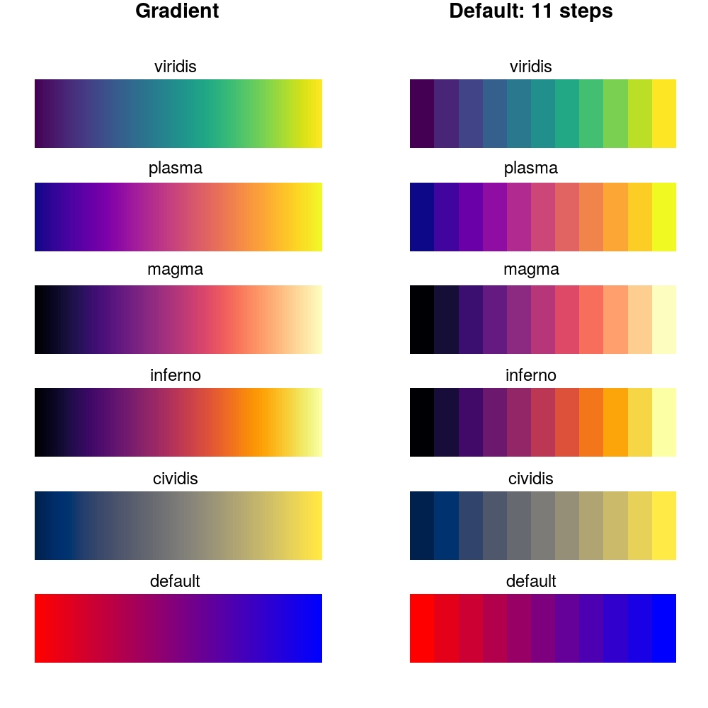
Color schemes
rtomahawk comes prepacked with a number of color schemes. Most of these are
taken directly from the
viridis R package and
are included here independent of that package to remove the package
interdependency. These color schemes are callable as functions taking as require
arguments the number of distinct values (n) and optionally the desired opacity
(alpha) level (alpha).
| Color scheme |
|---|
viridis |
plasma |
magma |
inferno |
cividis |
default |
We can plot these values as a gradient of values from [0, 100) and as [0, 11] by
calling the displayColors function:
1 | displayColors() |
Square representation
Graphically representing LD data is useful for checking data quality and in
exploration. If your data has already been loaded into memory using
readRecords it is possible to plot this data as individual data points using
the plotLD function. This approach is generally only feasable for visualizing
smaller genomic regions, for example, < 2-3 megabases. If you are investigating
longer ranges than this you should consider using the aggregation functions
provided in tomahawk/rtomahawk.
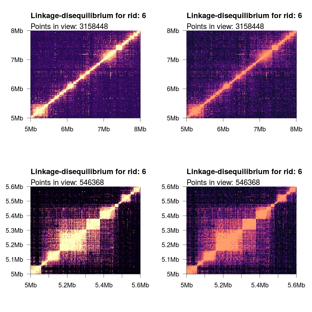
Because of the vast number of data points rendered and the finite amount of
pixels available, we render data points with an opacity gradient scaled
according to its R2 value from [0.1, 1]. This allows for mixing of both colors
and opacities to more clearly represent the distribution of the underlying data.
It is possible to disable this functionality by setting the optional argument
opacity to FALSE. In the following examples, we render both a large region
(5-8 Mb) and a small region (5.0-5.6 Mb) with and without the opacity flag set.
We also showcase the different color schemes.
1 2 3 4 5 6 7 8 9 10 11 | # Load some local data into memory. twk <- openTomahawkOutput("1kgp3_chr6.two") y <- readRecords(twk,"6:5e6-10e6", really=TRUE) # Plot two panels in the same figure. # Top panel: opacity gradient from [0.1, 1.0] mapping to # R2 range [0.1, 0.1, 0.2, ..., 1.0] # <COLOR> placeholder gets replaced with one of the color # schemes described below. par(mfrow=c(2,1)) plotLD(y, ylim=c(5e6,8e6), xlim=c(5e6,8e6), colors=<COLOR>, bg=<COLOR>(11)[1]) plotLD(y, ylim=c(5e6,8e6), xlim=c(5e6,8e6), colors=<COLOR>, bg=<COLOR>(11)[1], opacity=FALSE) |
| Color scheme | Image |
|---|---|
default |
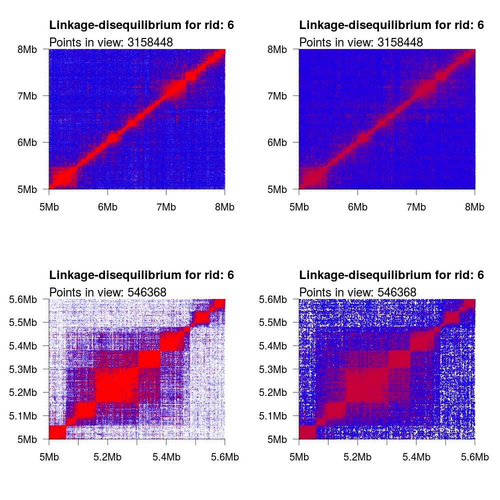 |
cividis |
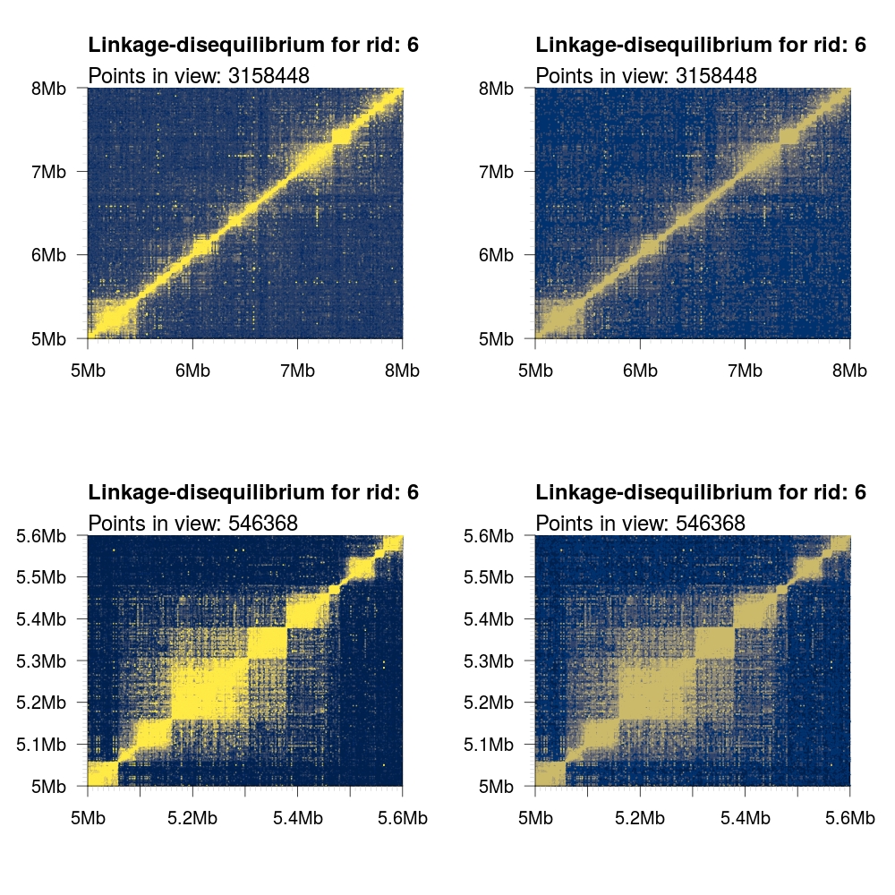 |
inferno |
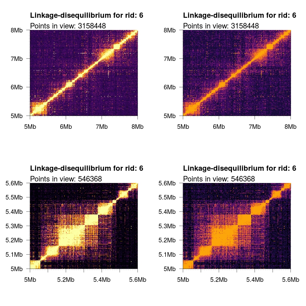 |
magma |
 |
plasma |
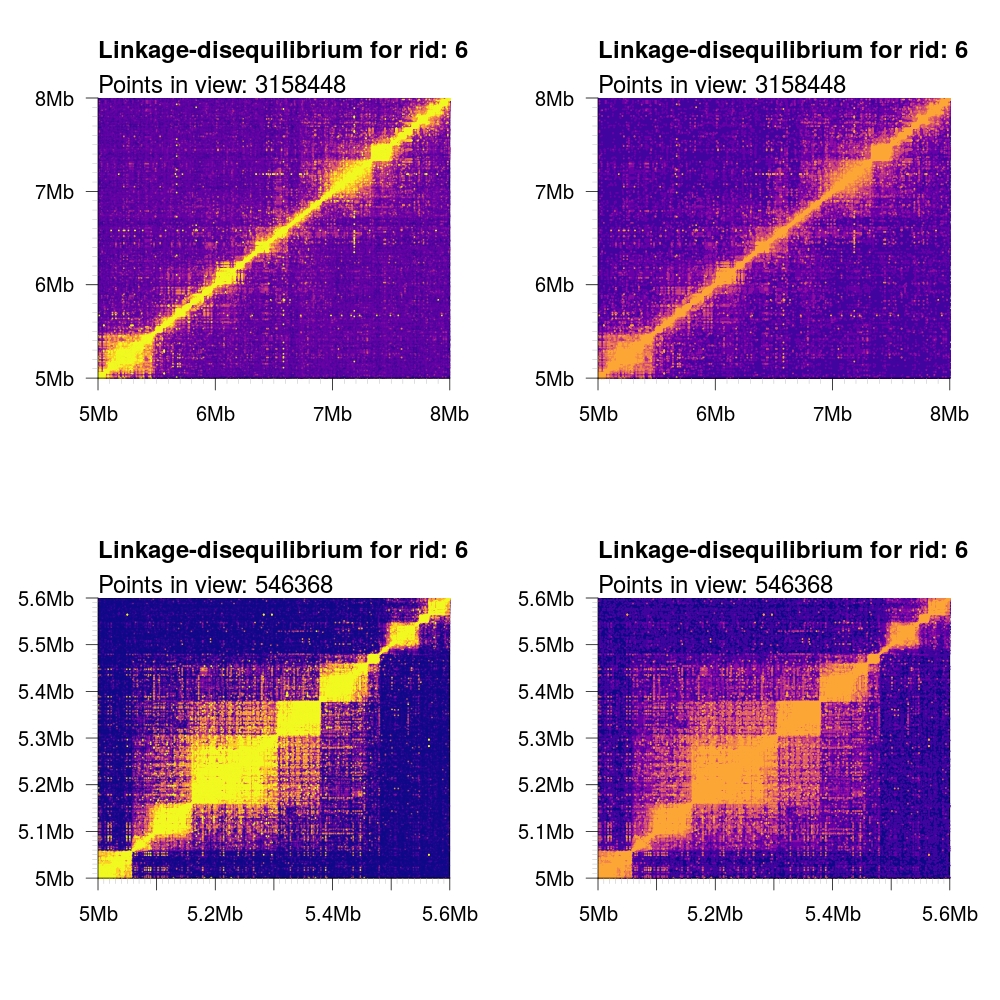 |
viridis |
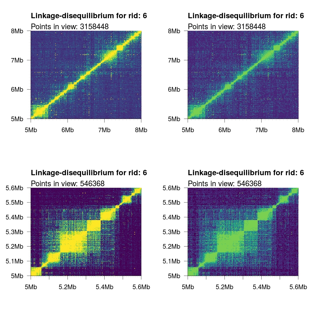 |
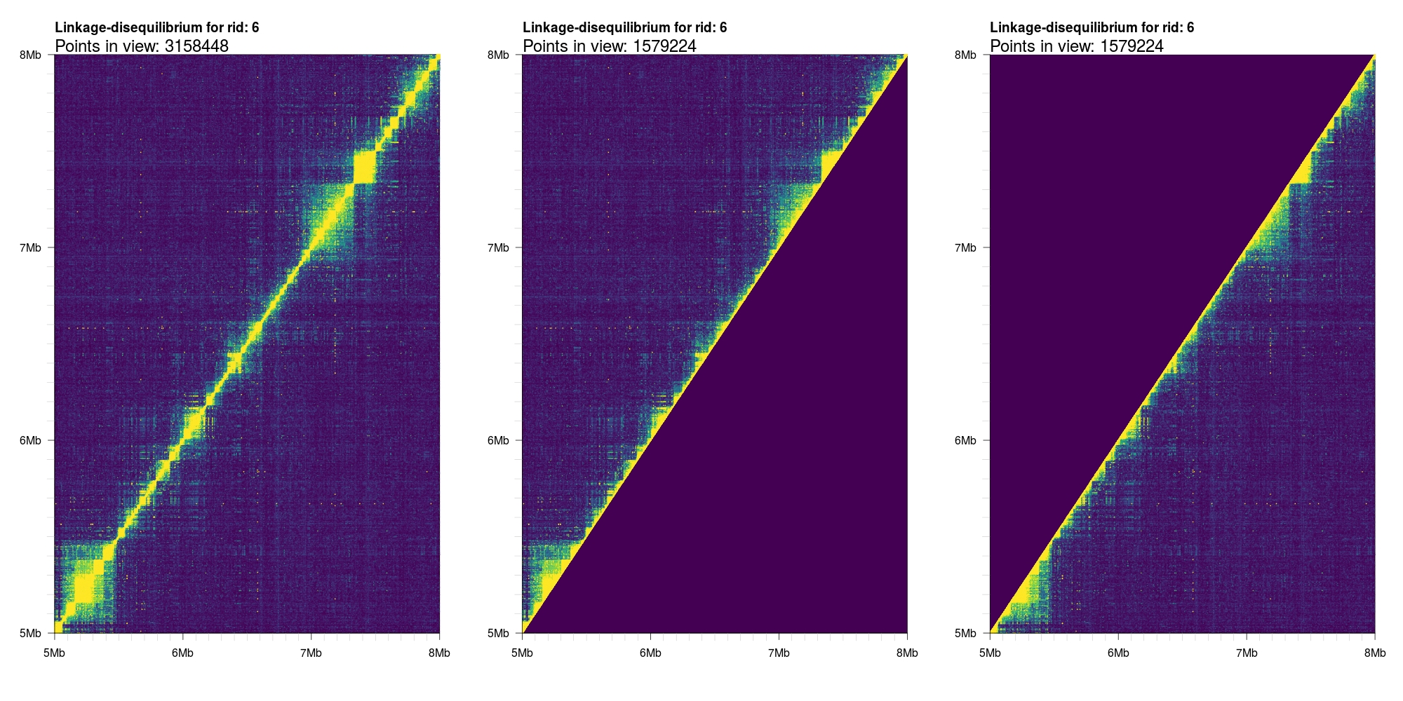
By default, the birectionally symmetric output data from tomahawk is kept (i.e. both (A,B) and (B,A))
tuples are kept. For this reason, the output plot will be square (or rectangular with mismatched xlim
and ylim parameters). In some cases, only the upper or lower triangular values are desired. We can
control what values are plotted with the logical upper and lower parameters.
1 2 3 4 | par(mfrow=c(1,3)) plotLD(y,ylim=c(5e6,8e6),xlim=c(5e6,8e6),colors=viridis(11),bg=viridis(11)[1]) plotLD(y,ylim=c(5e6,8e6),xlim=c(5e6,8e6),colors=viridis(11),bg=viridis(11)[1], upper=T) plotLD(y,ylim=c(5e6,8e6),xlim=c(5e6,8e6),colors=viridis(11),bg=viridis(11)[1], lower=T) |
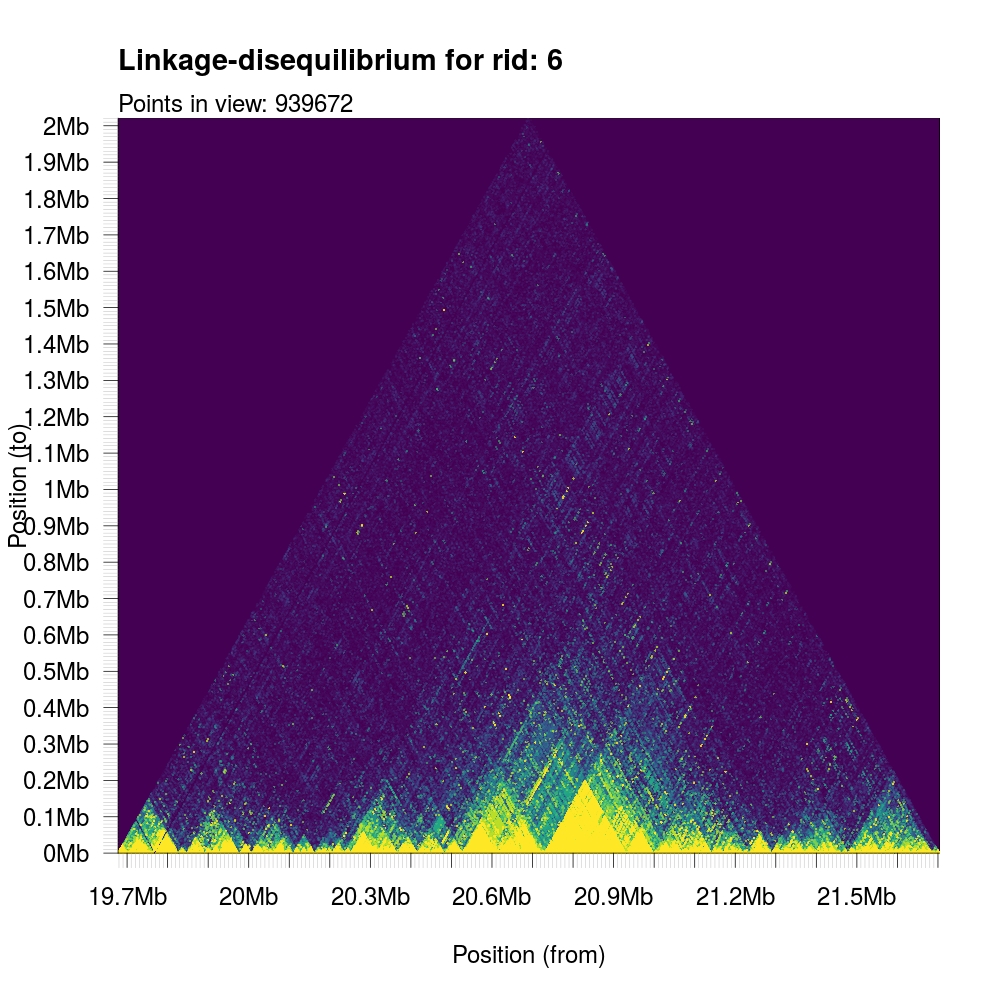
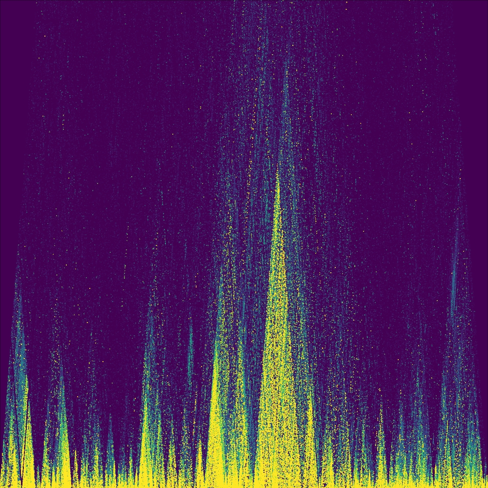
Triangular representation
In many cases, there is generally no need to graphically represent the entire
square (or rectangular) symmetric matrix of associations. This is especially
true when combining multiple graphs together to create a more comprehensive
picture of a particular region or feature. The topic of combining plots will be
explored in greter detail below. All of the examples here involves the
subroutine plotLDTriangular. As a design choice, we decided to restrict the
rendered y-axis data such that it is always bounded by the x-axis limits. For
this reason, these plots will always be triangular will partially "missing"
(omitted) values even if they are technically present in the dataset.
First, we describe its most basic use case. In the following example, we will
plot a section of associations with the viridis color palette and specifiy the
background to be the lowest (in this case, first) color in that scheme.
1 | plotLDTriangular(y,colors=viridis(11),bg=viridis(11)[1]) |
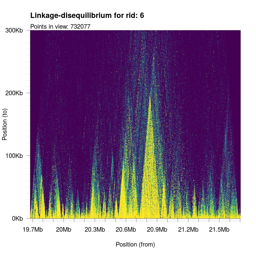
Because of the smallish haplotype blocks in humans, most of these visible triangular structures will have limited span in the y-axis. We can truncate the y-axis to zoom into the local neighbourhood and more accurately display the local haplotype structure.
1 | plotLDTriangular(y,colors=viridis(11),bg=viridis(11)[1],ylim=c(0,300e3)) |
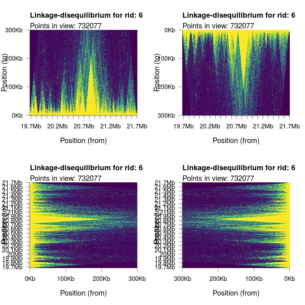
It is possible to control the orientation (rotation) of the output graph by
specifying the orientation parameter. The numerial encodings are: 1)
standard; 2) upside down;
3) left-right flipped; and 4) right-left flipped.
1 2 3 4 5 | par(mfrow=c(2,2)) plotLDTriangular(y,ylim=c(0,300e3),colors=viridis(11),bg=viridis(11)[1], orientation = 1) plotLDTriangular(y,ylim=c(0,300e3),colors=viridis(11),bg=viridis(11)[1], orientation = 2) plotLDTriangular(y,ylim=c(0,300e3),colors=viridis(11),bg=viridis(11)[1], orientation = 3) plotLDTriangular(y,ylim=c(0,300e3),colors=viridis(11),bg=viridis(11)[1], orientation = 4) |
It is possible to completely disable all anotation by setting the logical
parameter annotate to FALSE. This will remove titles, axes, and ticks.
1 | plotLDTriangular(y,ylim=c(0,300e3),colors=viridis(11),bg=viridis(11)[1], orientation = 1, annotate = FALSE) |
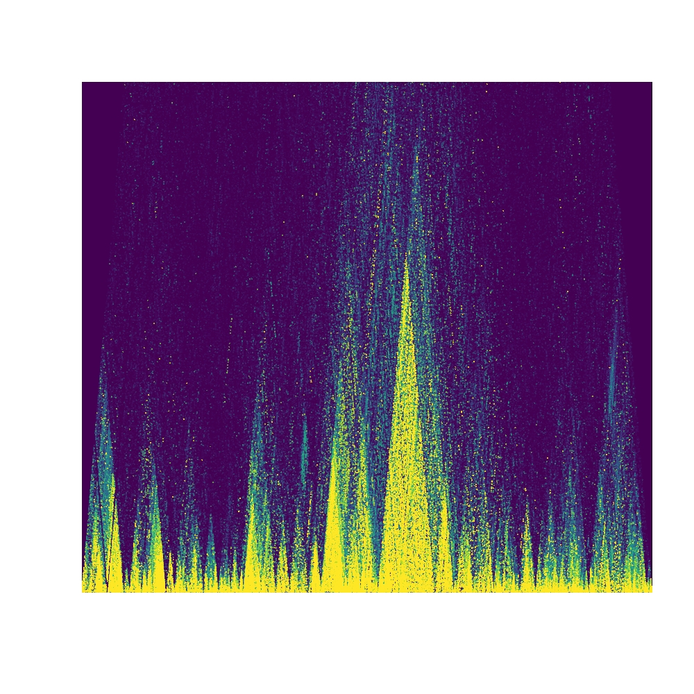
Note that these plotting functions respect the global mar (margin) values and
(by default) will have white space around it. We can change the global par
argument to, for example, zero to remove these margins when annotation is
disabled for edge-to-edge graphics.
Visualizing GWAS data and LD
In this section we will produce LocusZoom-like plots using GWAS data from the UK BioBank comprised exclusively of white British individuals. The Roslin Institute at the University of Edinbrugh host a data browser of associatins called Gene Atlas. In the following examples we will investigate the association of genotypes at chromosome 6 and diabetes in this cohort. Data in its entirety can be explored further using the Gene Atlas. To reproduce the results below download the imputed data for chromosome 6 and the associated positional information.
1 2 3 4 5 6 7 8 9 10 11 12 13 14 15 16 17 18 19 20 21 22 23 24 25 | # Downloaded data from: # http://static.geneatlas.roslin.ed.ac.uk/gwas/allWhites/imputed/data.copy/imputed.allWhites.selfReported_n_1245.chr6.csv.gz # http://static.geneatlas.roslin.ed.ac.uk/gwas/allWhites/snps/extended/snps.imputed.chr6.csv.gz library(data.table) # For speedier reading of data. # We zcat (uncompress gzipped archive) directly into fread. # This may not work for Windows users. In that case, decompress # the files manually first. x <- fread("zcat imputed.allWhites.selfReported_n_1245.chr6.csv.gz", sep=" ") snp <- fread("zcat snps.imputed.chr6.csv.gz", sep=" ") # Keep matching data available in both files. We neeed to maintain # parity between the two sets. snp <- snp[match(x$SNP, snp$SNP),] # Transform linear-scale (untransformed) P-values into -log10(P). snp$p <- -log10(x$`PV-selfReported_n_1245`) # Setup path to local Tomahawk file to compute LD against. twk2 <- new("twk") twk2@file.path <- "1kgp3_chr6.twk" # Load human recombination data (hg19) supplied with `rtomahawk` data(gmap) # Region of 1 Mb in either direction of target. single <- plotLZ(twk2, "6:20694884", snp, gmap, window=1e6, minR2=0) # Region of 50 Kb in either direction of target. single <- plotLZ(twk2, "6:20694884", snp, gmap, window=50e3, minR2=0) |
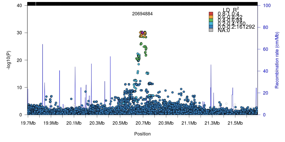
Internal LD computation
The plotLZ plotting function will internally compute linkage-disequilibrium
for a target SNV and it's surrounding genomic region. This background computation
is stored in a temporary file and then loaded back into memory and returned as a new
twk class instance. If you have further use of this information then you
need to capture the return value of this function. It is possible to change the
default temp directory used in R with the subroutine set.tempdir. Please note
that all data written to this temporary directory will be purged upon exiting the
current session of R.
These functions are extremely fast as the R-bindings use .Call commands to
communicate with the compiled C++ shared object:
1 2 3 4 5 6 7 | > system.time(plotLZ(twk2, "6:20694884", snp, gmap, window=1e6, minR2=0)) user system elapsed 1.405 0.001 1.407 > system.time(plotLZ(twk2, "6:20694884", snp, gmap, window=50e3, minR2=0)) user system elapsed 0.115 0.004 0.119 |
Almost all of this time is spent rendering symbols in the vectorized plot. The same command using the CLI takes roughly 1/3rd of the time:
1 2 3 4 | $ time tomahawk scalc -i 1kgp3_chr6.twk -I 6:20694884 -w 1000000 > /dev/null real 0m0.452s user 0m0.937s sys 0m0.061s |
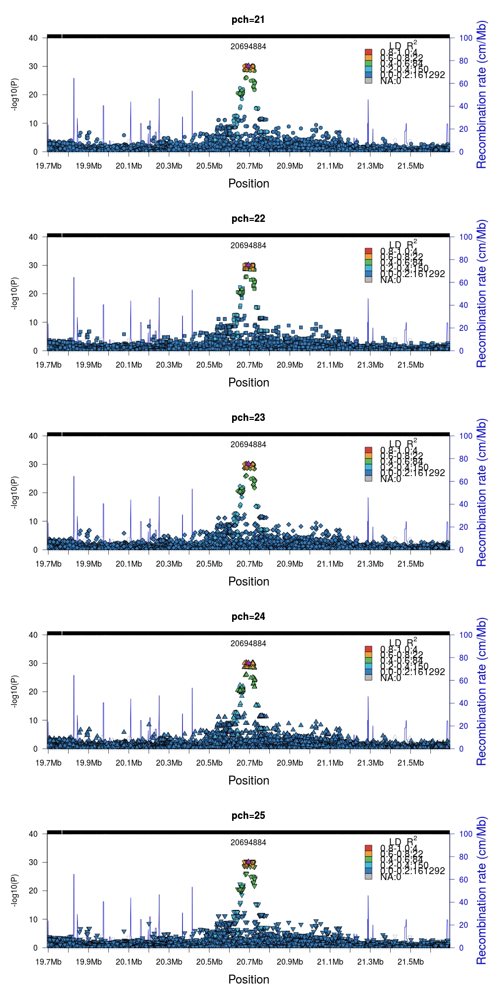
Many aspects of the plots can be customized to your needs. For example,
modifying the datapoint symbol pch in the valid range [21, 25]. Note that all
other pch values are technically valid but will not generate a fill color.
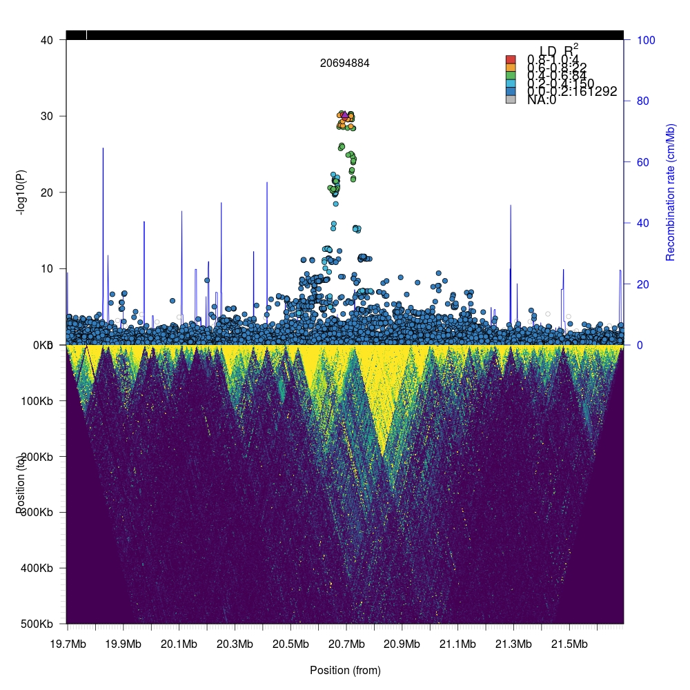
If your visualizations require additional data layers it is possible to combine
these into a single plot as rtomahawk renders plots using base-R. In this
example we will combine two plots generated by rtomahawk: the GWAS P-value and
its single-site LD together with the all-vs-all pairwise LD for the same region.
1 2 3 4 5 6 | par(mfrow=c(2,1), mar=c(0,5,3,5)) # Set bottom margin to 0. single <- plotLZ(twk2, "6:20694884", snp, gmap, window=1e6, minR2=0, xlab="", xaxt="n") twk <- openTomahawkOutput("test_region.two") y <- readRecords(twk, really=TRUE) par(mar=c(5,5,0,5)) # Set top margin to 0. plotLDTriangular(y, ylim=c(0,500e3), xlim=c(20694884 - 1e6, 20694884 + 1e6), colors=viridis(11), bg=viridis(11)[1], orientation = 2, cex=.25, main="") |
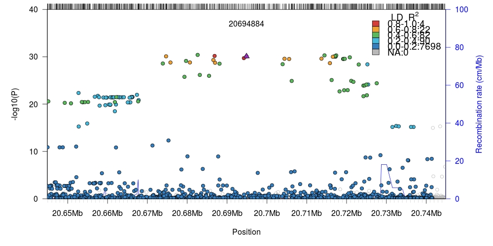
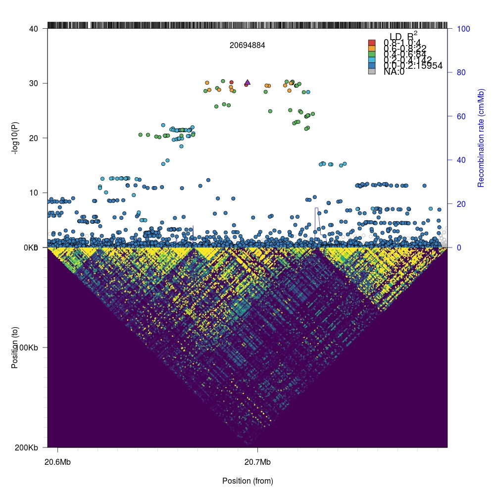
We can zoom into the local region (100kb flanking region) by simply changing the
window parameter in plotLZ and the xlim range in plotLDTriangular.
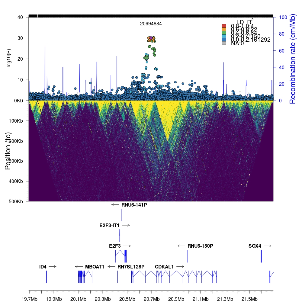
It is possible to add more advanced data layers using external packages with
some simple manipulations. In this example we will add a gene track using
genetic information extracted from biomaRt and drawn using Sushi, both
third-party packages.
biomaRt information
The R package biomaRt requires internet connectivity to function as the
package itself is a wrapper around the Ensembl BioMart
tool that allows extraction of connected data from databases without having
to perform explicit programming.
1 2 3 4 5 6 7 8 9 10 11 12 13 14 15 16 17 18 19 20 21 22 23 24 25 26 27 28 29 30 31 32 33 34 35 36 37 38 39 40 41 42 43 | library(biomaRt) mart <- useMart(host='http://grch37.ensembl.org',biomart="ensembl", dataset="hsapiens_gene_ensembl") # We will retrieve results from biomaRt twice because the database # does _not_ allow simultaneous queries for exon-level data and # gene-level data. To overcome this problem, we will perform two # quries to the database and merge the results together. results <- getBM(attributes = c("ensembl_exon_id", "exon_chrom_start","exon_chrom_end"), filters = c("chromosome_name", "start", "end"), values=list(6, 20694884-1e6, 20694884+1e6), mart=mart) results2 <- getBM(attributes = c("ensembl_exon_id","hgnc_symbol", "chromosome_name", "start_position", "end_position","strand"), filters = c("chromosome_name", "start", "end"), values=list(6, 20694884-1e6, 20694884+1e6), mart=mart) results<-cbind(results,results2[,-1,drop=F]) results<-results[results$hgnc_symbol!="",] results<-results[,c(2,3,4,5,8)] names(results) <- c("start","stop","gene","chrom","strand") results$score = "." results<-results[,c("chrom","start","stop","gene","score", "strand")] library(Sushi) chrom = 6 chromstart = 20694884-1e6 chromend = 20694884+1e6 layout(matrix(1:3,ncol=1),heights = c(2,2,1)) par(mar=c(0,5,3,5)) # Set bottom margin to 0. single <- plotLZ(twk2, "6:20694884", snp, gmap, window=1e6, minR2=0, xlab="", xaxt="n") twk<-openTomahawkOutput("test_region.two") y<-readRecords(twk,really=TRUE) par(mar=c(0,5,0,5)) # Set top and bottom margins to 0. plotLDTriangular(y, ylim=c(0,500e3), xlim=c(20694884 - 1e6, 20694884 + 1e6), colors=viridis(11), bg=viridis(11)[1], orientation = 2, cex=.25, main="") par(mar=c(2,5,0,5)) plotGenes(geneinfo=results, chrom=chrom, chromstart=chromstart, chromend=chromend, labeloffset=.5, fontsize=1, arrowlength = 0.025) abline(v=20694884,lty="dashed",col="grey") # Highjack internal `rtomahawk` function for drawing genomic axes. # This function is unexported and is not intended for general use. rtomahawk:::addGenomicAxis(c(chromstart,chromend),at = 1, las = 1, F) |
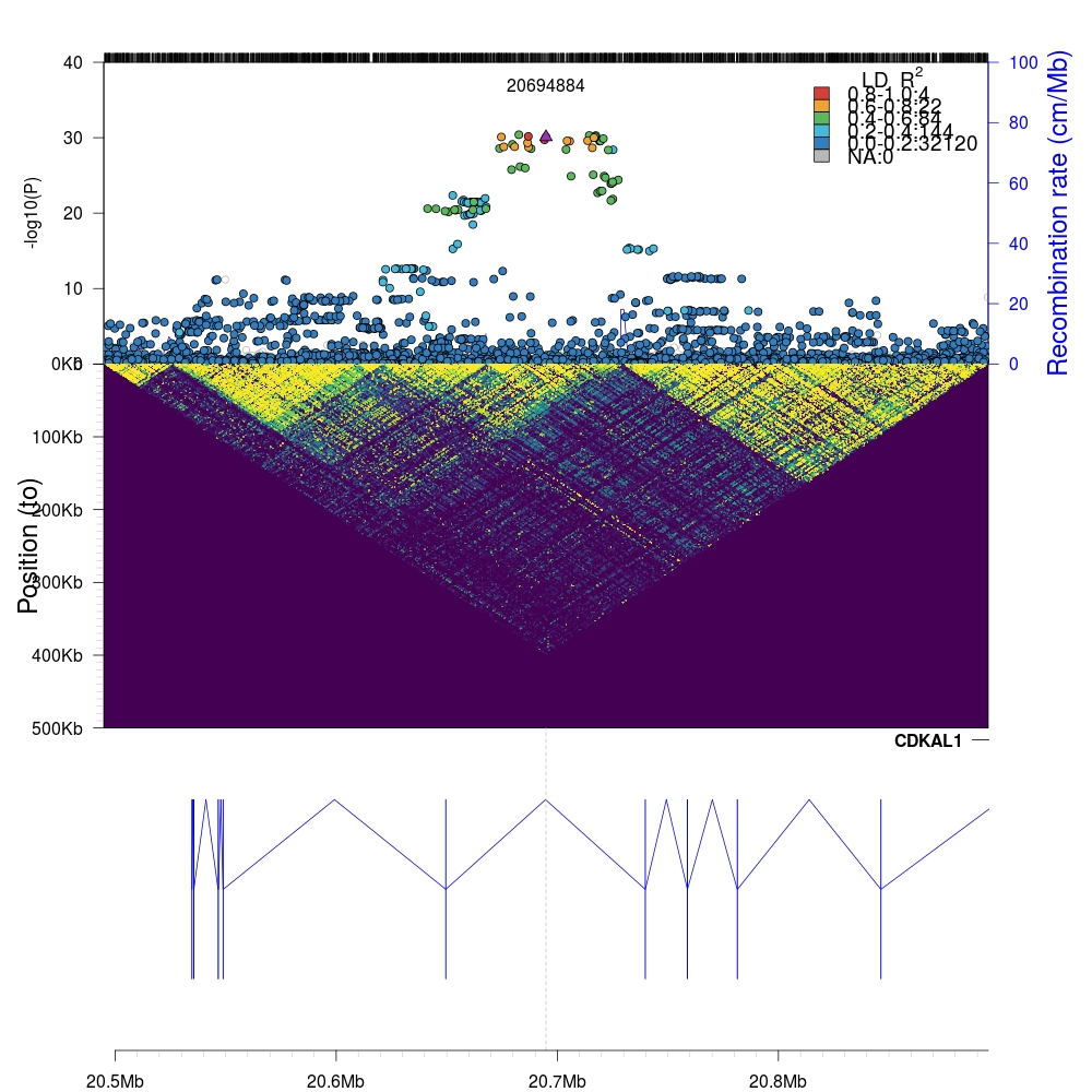
Again, we can zoom into the local region (200kb flanking region) by simply changing the appropriate parameters in the code above.
The plotting time can vary from milliseconds to several seconds depending on the
number of points that are being computed directly (top panel) and the number of
points that are loaded and rendered (middle panel). In the first example above,
rtomahawk and tomahawk computes and plots millions of LD associations and
data points in a few seconds on a single thread.
1 2 3 | > system.time(f()) user system elapsed 6.336 0.260 6.233 |
In this code snippet, the function f(), is simply a placeholder for the code
above.
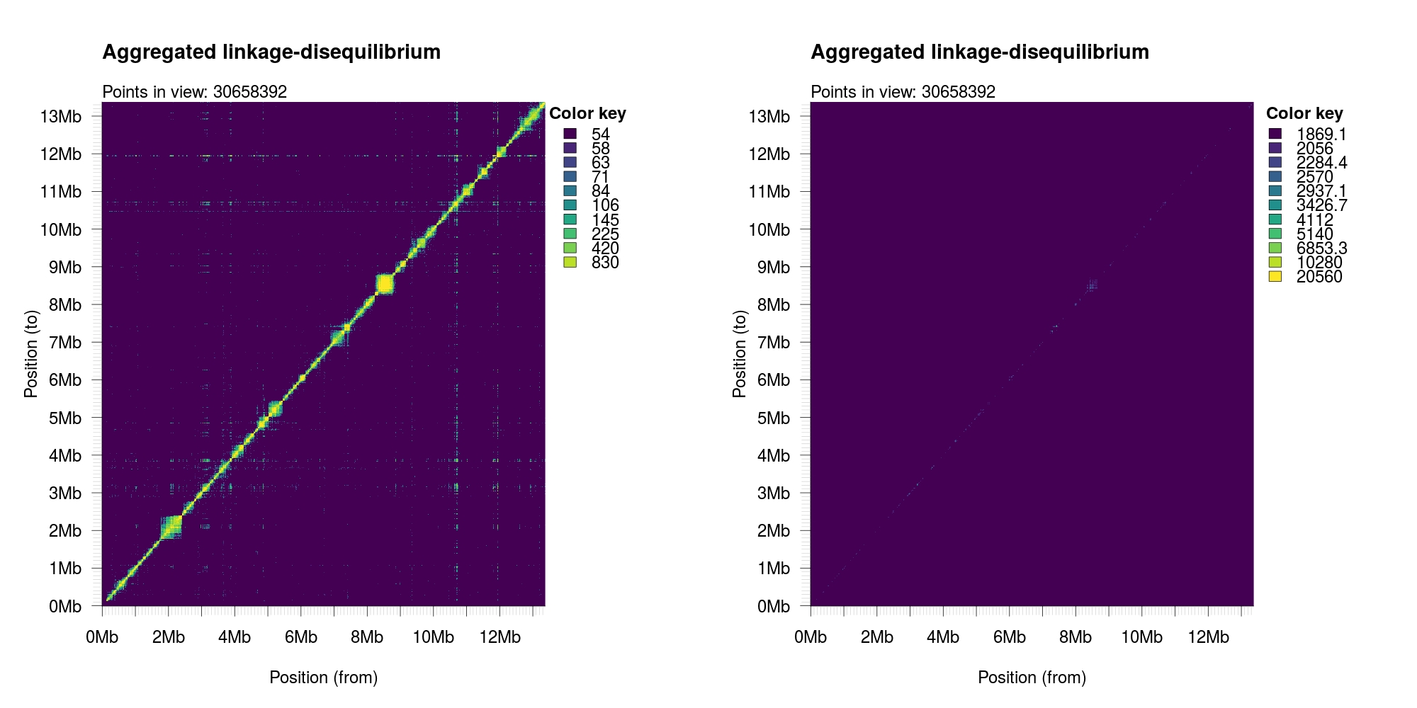
Aggregating and visualizing datasets
Quantile-normalized (left) or linear range (right)
Unsafe method
In the current release of rtomahawk, this subroutine does not check for
user-interruption (for example Ctrl+C or Ctrl+Z) commands. This means that
you need to wait until the underlying process has finished or you have to
terminate the host R session, in turn killing the spawned process. This will
be fixed in upcoming releases.
1 2 3 4 5 | twk<-openTomahawkOutput("example.two") x<-aggregate(twk,aggregation="r2", reduction="count",xbins=1000, ybins=1000,minCount=50, verbose=T, threads=8) par(mar=c(5,5,5,8), mfrow=c(1,2)) plotAggregation(x, normalize = TRUE) plotAggregation(x, normalize = FALSE) |
1 2 3 4 5 6 7 8 9 10 11 12 13 14 15 16 17 18 | > agg <- aggregate(twk,"r2", "count", 1000, 1000, 50, verbose=T, threads=6) Program: tomahawk-062954eb (Tools for computing, querying and storing LD data) Libraries: tomahawk-0.7.0; ZSTD-1.3.1; htslib 1.9 Contact: Marcus D. R. Klarqvist <mk819@cam.ac.uk> Documentation: https://github.com/mklarqvist/tomahawk License: MIT ---------- [2019-01-19 11:05:37,072][LOG] Calling aggregate... [2019-01-19 11:05:37,072][LOG] Performing 2-pass over data... [2019-01-19 11:05:37,072][LOG] ===== First pass (peeking at landscape) ===== [2019-01-19 11:05:37,072][LOG] Blocks: 32 [2019-01-19 11:05:37,072][LOG] Uncompressed size: 5.286261 Gb [2019-01-19 11:05:37,072][LOG][THREAD] Data/thread: 881.043564 Mb [2019-01-19 11:05:41,040][LOG] ===== Second pass (building matrix) ===== [2019-01-19 11:05:41,040][LOG] Aggregating 49,870,388 records... [2019-01-19 11:05:41,040][LOG][THREAD] Allocating: 240.000000 Mb for matrices... [2019-01-19 11:05:44,797][LOG] Aggregated 49,870,388 records in 1,000,000 bins. [2019-01-19 11:05:44,798][LOG] Finished. |
Load a pre-computed tomahawk aggregation object:
1 | agg <- loadAggregate("agg.twa") |